※本ページの内容はテキストの第6章に相当します
変数間の関係を調べる方法は変数の種類により下記の三つの組み合わせにより決まります。
- {量的変数, 量的変数}
- 散布図・相関係数
- {質的変数, 質的変数}
- 分割表・独立性の検定
- {量的変数, 質的変数}
- 量的変数の層別解析
本章ではRcmdrで実行した場合のコードと出力結果のみを記載し、手順の記載は省略しますので詳細はテキストを参照してください。
データの読み込み
- Rcmdrのメニューから[データ]-[データセットのロード…]を実行する
- ファイルダイアログで「
外来患者ストレス.RData」ファイルを選択する - アクティブデータセットが
PatientStressになっていることを確認する
6.1 複数の量的変数間の関連性(P113-)
6.1.1 散布図(P113-P117)
グラフ - 散布図
car::scatterplot(ストレス反応~日常苛立ちごと, regLine=TRUE,
                 smooth=list(span=0.5, spread=TRUE), boxplots=FALSE,
                 jitter=list(x=1),
                 data=PatientStress)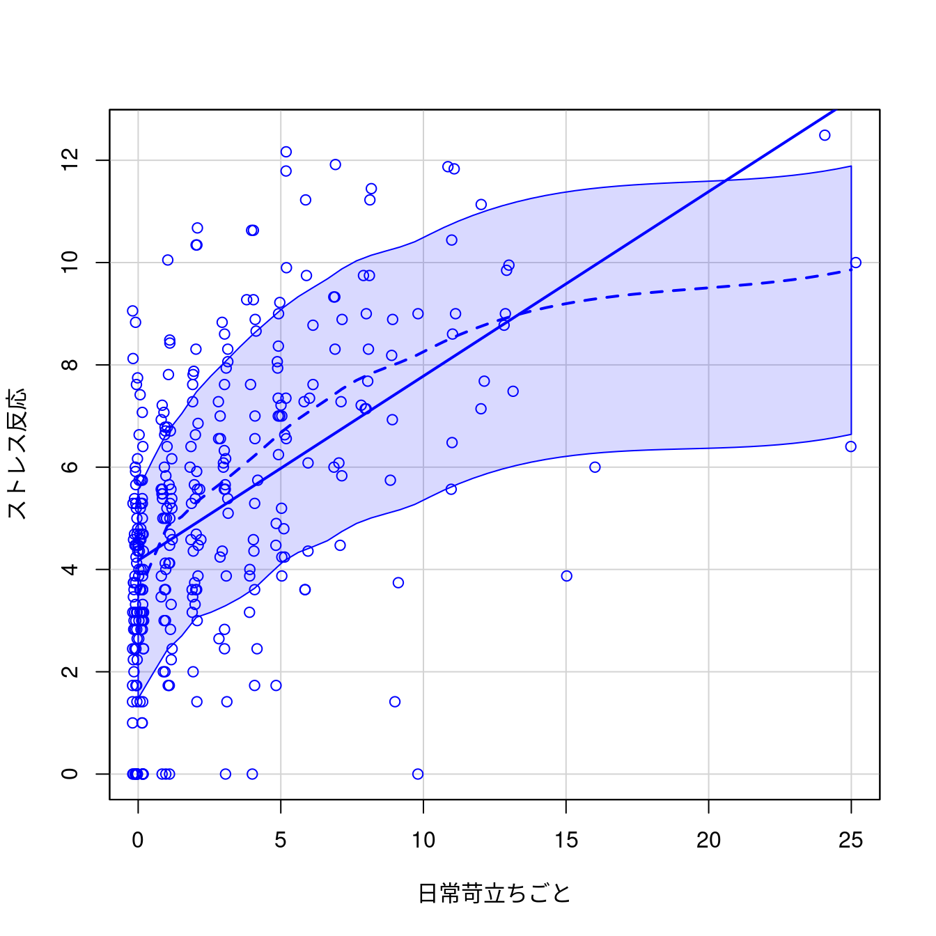
グラフ - 散布図
car::scatterplot(ストレス反応~日常苛立ちごと | 性別, regLine=TRUE,
                 smooth=list(span=0.5, spread=TRUE), boxplots=FALSE,
                 jitter=list(x=1), by.groups=TRUE,
                 legend=list(coords="bottomright"), data=PatientStress)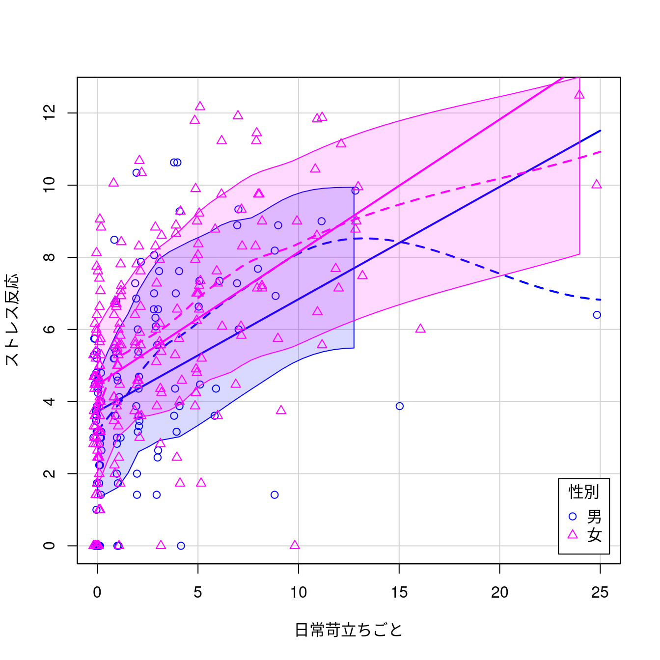
6.1.2 相関の検定(P118-P123)
6.1.3 散布図行列(P123-P126)
グラフ - 散布図行列
car::scatterplotMatrix(~ストレス反応+ストレッサー得点+健康統制感,
                       regLine=TRUE, smooth=list(span=0.5, spread=FALSE),
                       diagonal=list(method="histogram"),
                       data=PatientStress)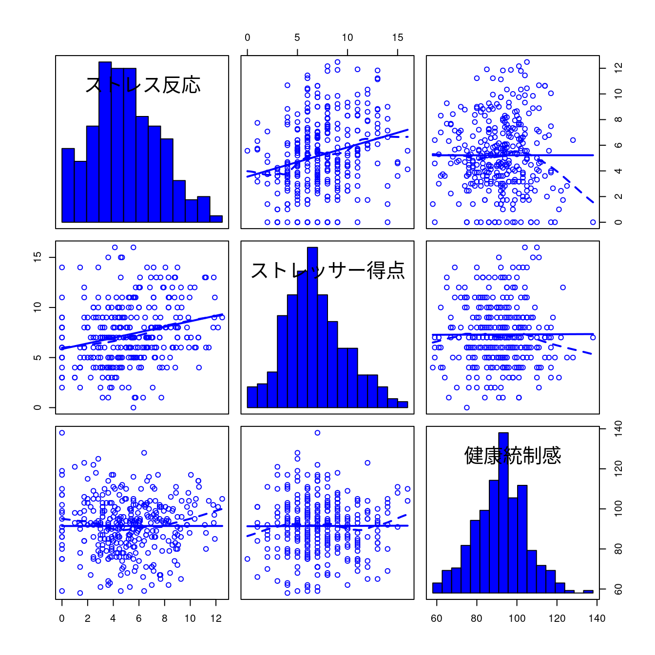
6.1.4 相関の検定
統計量 - 要約 - 相関の検定
RcmdrMisc::rcorr.adjust(
  PatientStress[,c("ストレス反応","ストレッサー得点","健康統制感")],
  type="pearson", use="complete")
Pearson correlations:
ストレス反応 ストレッサー得点 健康統制感
ストレス反応 1.0000 0.2515 3e-04
ストレッサー得点 0.2515 1.0000 4e-03
健康統制感 0.0003 0.0040 1e+00
Number of observations: 337
Pairwise two-sided p-values:
ストレス反応 ストレッサー得点 健康統制感
ストレス反応 <.0001 0.9962
ストレッサー得点 <.0001 0.9419
健康統制感 0.9962 0.9419
Adjusted p-values (Holm's method)
ストレス反応 ストレッサー得点 健康統制感
ストレス反応 <.0001 1
ストレッサー得点 <.0001 1
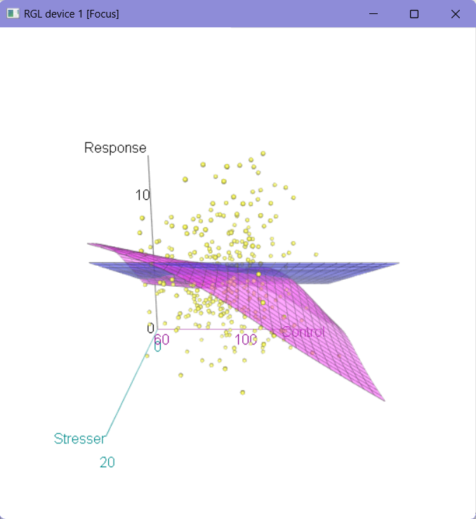
健康統制感 1 1 6.1.5 3次元散布図(鳥瞰図)(P126-P130)
本環境では実行できませんのでスクリーンショットで代用します。
6.2 複数の質的変数間の関連性(P130-)
6.2.1 2元分割表(P130-P136)
統計量 - 分割表 - 2元表
local({
  .Table <- xtabs(~日常苛立ち+ノンコンプライアンス, data=PatientStress)
  cat("\nFrequency table:\n")
  print(.Table)
  cat("\nRow percentages:\n")
  print(RcmdrMisc::rowPercents(.Table))
  .Test <- chisq.test(.Table, correct=FALSE)
  print(.Test)
})
Frequency table:
          ノンコンプライアンス
日常苛立ち なし あり
         0   79   39
         1   55   34
         3   34   38
         6   34   24

Row percentages:
          ノンコンプライアンス
日常苛立ち なし あり Total Count
         0 66.9 33.1   100   118
         1 61.8 38.2   100    89
         3 47.2 52.8   100    72
         6 58.6 41.4   100    58

    Pearson's Chi-squared test

data:  .Table
X-squared = 7.4341, df = 3, p-value = 0.05928
統計量 - 分割表 - 2元表
local({
  .Table <- xtabs(~性別+ノンコンプライアンス, data=PatientStress)
  cat("\nFrequency table:\n")
  print(.Table)
  cat("\nRow percentages:\n")
  print(RcmdrMisc::rowPercents(.Table))
  .Test <- chisq.test(.Table, correct=FALSE)
  print(.Test)
  cat("\nExpected counts:\n")
  print(.Test$expected)
  print(fisher.test(.Table))
})
Frequency table:
    ノンコンプライアンス
性別 なし あり
  男   68   51
  女  134   84

Row percentages:
    ノンコンプライアンス
性別 なし あり Total Count
  男 57.1 42.9   100   119
  女 61.5 38.5   100   218

    Pearson's Chi-squared test

data:  .Table
X-squared = 0.59969, df = 1, p-value = 0.4387


Expected counts:
    ノンコンプライアンス
性別      なし     あり
  男  71.32938 47.67062
  女 130.67062 87.32938

    Fisher's Exact Test for Count Data

data:  .Table
p-value = 0.4856
alternative hypothesis: true odds ratio is not equal to 1
95 percent confidence interval:
 0.5180684 1.3524537
sample estimates:
odds ratio
 0.8362745
6.2.2 多元分割表(P136-P139)
統計量 - 分割表 - 多元表
Frequency table:
, , 性別 = 男

          ノンコンプライアンス
日常苛立ち なし あり
         0   28   19
         1   17   15
         3   12   12
         6   11    5

, , 性別 = 女

          ノンコンプライアンス
日常苛立ち なし あり
         0   51   20
         1   38   19
         3   22   26
         6   23   19


Row percentages:
, , 性別 = 男

          ノンコンプライアンス
日常苛立ち なし あり Total Count
         0 59.6 40.4   100    47
         1 53.1 46.9   100    32
         3 50.0 50.0   100    24
         6 68.8 31.2   100    16

, , 性別 = 女

          ノンコンプライアンス
日常苛立ち なし あり Total Count
         0 71.8 28.2   100    71
         1 66.7 33.3   100    57
         3 45.8 54.2   100    48
         6 54.8 45.2   100    42
統計量 - 分割表 - 2元表
local({
  .Table <- xtabs(~日常苛立ち+ノンコンプライアンス, data=PatientStress,
                  subset=性別=="女")
  cat("\nFrequency table:\n")
  print(.Table)
  cat("\nRow percentages:\n")
  print(RcmdrMisc::rowPercents(.Table))
  .Test <- chisq.test(.Table, correct=FALSE)
  print(.Test)
})
Frequency table:
          ノンコンプライアンス
日常苛立ち なし あり
         0   51   20
         1   38   19
         3   22   26
         6   23   19

Row percentages:
          ノンコンプライアンス
日常苛立ち なし あり Total Count
         0 71.8 28.2   100    71
         1 66.7 33.3   100    57
         3 45.8 54.2   100    48
         6 54.8 45.2   100    42

    Pearson's Chi-squared test

data:  .Table
X-squared = 9.6211, df = 3, p-value = 0.02208